


Logical Data Modeling
Now that you have defined your queries, you’re ready to begin designing Cassandra tables. First, create a logical model containing a table for each query, capturing entities and relationships from the conceptual model.
To name each table, you’ll identify the primary entity type for which
you are querying and use that to start the entity name. If you are
querying by attributes of other related entities, append those to the
table name, separated with by. For example, hotels_by_poi.
Next, you identify the primary key for the table, adding partition key columns based on the required query attributes, and clustering columns in order to guarantee uniqueness and support desired sort ordering.
The design of the primary key is extremely important, as it will determine how much data will be stored in each partition and how that data is organized on disk, which in turn will affect how quickly Cassandra processes reads.
Complete each table by adding any additional attributes identified by the query. If any of these additional attributes are the same for every instance of the partition key, mark the column as static.
Now that was a pretty quick description of a fairly involved process, so it will be worthwhile to work through a detailed example. First, let’s introduce a notation that you can use to represent logical models.
Several individuals within the Cassandra community have proposed notations for capturing data models in diagrammatic form. This document uses a notation popularized by Artem Chebotko which provides a simple, informative way to visualize the relationships between queries and tables in your designs. This figure shows the Chebotko notation for a logical data model.
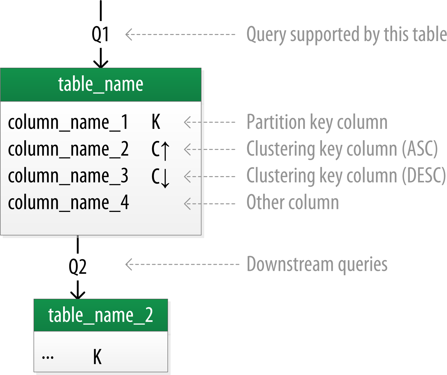
Each table is shown with its title and a list of columns. Primary key columns are identified via symbols such as K for partition key columns and C↑ or C↓ to represent clustering columns. Lines are shown entering tables or between tables to indicate the queries that each table is designed to support.
Hotel Logical Data Model
The figure below shows a Chebotko logical data model for the queries involving hotels, points of interest, rooms, and amenities. One thing you’ll notice immediately is that the Cassandra design doesn’t include dedicated tables for rooms or amenities, as you had in the relational design. This is because the workflow didn’t identify any queries requiring this direct access.
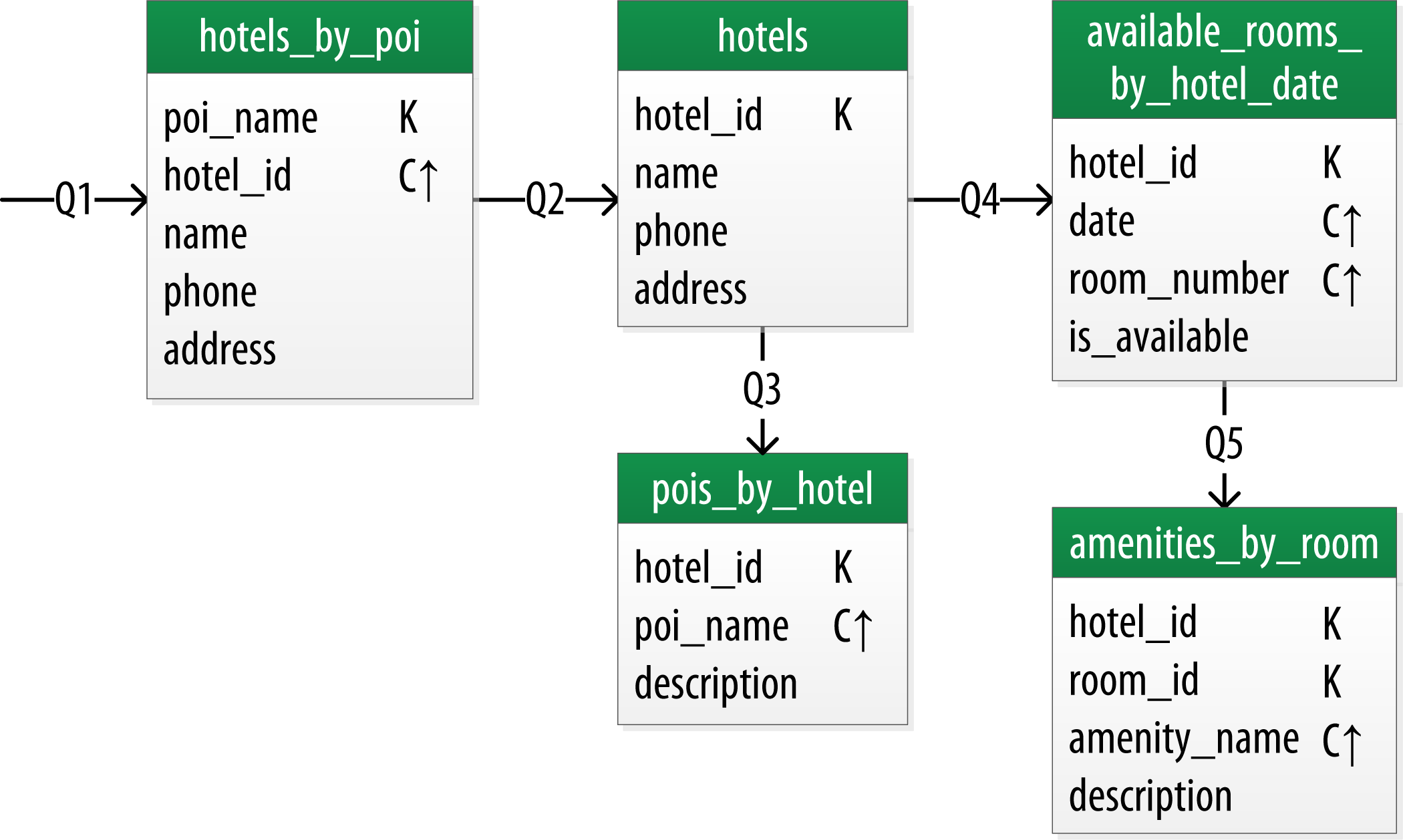
Let’s explore the details of each of these tables.
The first query Q1 is to find hotels near a point of interest, so you’ll
call this table hotels_by_poi. Searching by a named point of interest
is a clue that the point of interest should be a part of the primary
key. Let’s reference the point of interest by name, because according to
the workflow that is how users will start their search.
You’ll note that you certainly could have more than one hotel near a given point of interest, so you’ll need another component in the primary key in order to make sure you have a unique partition for each hotel. So you add the hotel key as a clustering column.
An important consideration in designing your table’s primary key is making sure that it defines a unique data element. Otherwise you run the risk of accidentally overwriting data.
Now for the second query (Q2), you’ll need a table to get information
about a specific hotel. One approach would have been to put all of the
attributes of a hotel in the hotels_by_poi table, but you added only
those attributes that were required by the application workflow.
From the workflow diagram, you know that the hotels_by_poi table is
used to display a list of hotels with basic information on each hotel,
and the application knows the unique identifiers of the hotels returned.
When the user selects a hotel to view details, you can then use Q2,
which is used to obtain details about the hotel. Because you already
have the hotel_id from Q1, you use that as a reference to the hotel
you’re looking for. Therefore the second table is just called hotels.
Another option would have been to store a set of poi_names in the
hotels table. This is an equally valid approach. You’ll learn through
experience which approach is best for your application.
Q3 is just a reverse of Q1—looking for points of interest near a hotel,
rather than hotels near a point of interest. This time, however, you
need to access the details of each point of interest, as represented by
the pois_by_hotel table. As previously, you add the point of interest
name as a clustering key to guarantee uniqueness.
At this point, let’s now consider how to support query Q4 to help the
user find available rooms at a selected hotel for the nights they are
interested in staying. Note that this query involves both a start date
and an end date. Because you’re querying over a range instead of a
single date, you know that you’ll need to use the date as a clustering
key. Use the hotel_id as a primary key to group room data for each
hotel on a single partition, which should help searches be super fast.
Let’s call this the available_rooms_by_hotel_date table.
To support searching over a range, use clustering columns
<clustering-columns> to store attributes that you need to access in a
range query. Remember that the order of the clustering columns is
important.
The design of the available_rooms_by_hotel_date table is an instance
of the wide partition pattern. This pattern is sometimes called the
wide row pattern when discussing databases that support similar
models, but wide partition is a more accurate description from a
Cassandra perspective. The essence of the pattern is to group multiple
related rows in a partition in order to support fast access to multiple
rows within the partition in a single query.
In order to round out the shopping portion of the data model, add the
amenities_by_room table to support Q5. This will allow users to view
the amenities of one of the rooms that is available for the desired stay
dates.
Reservation Logical Data Model
Now let’s switch gears to look at the reservation queries. The figure shows a logical data model for reservations. You’ll notice that these tables represent a denormalized design; the same data appears in multiple tables, with differing keys.
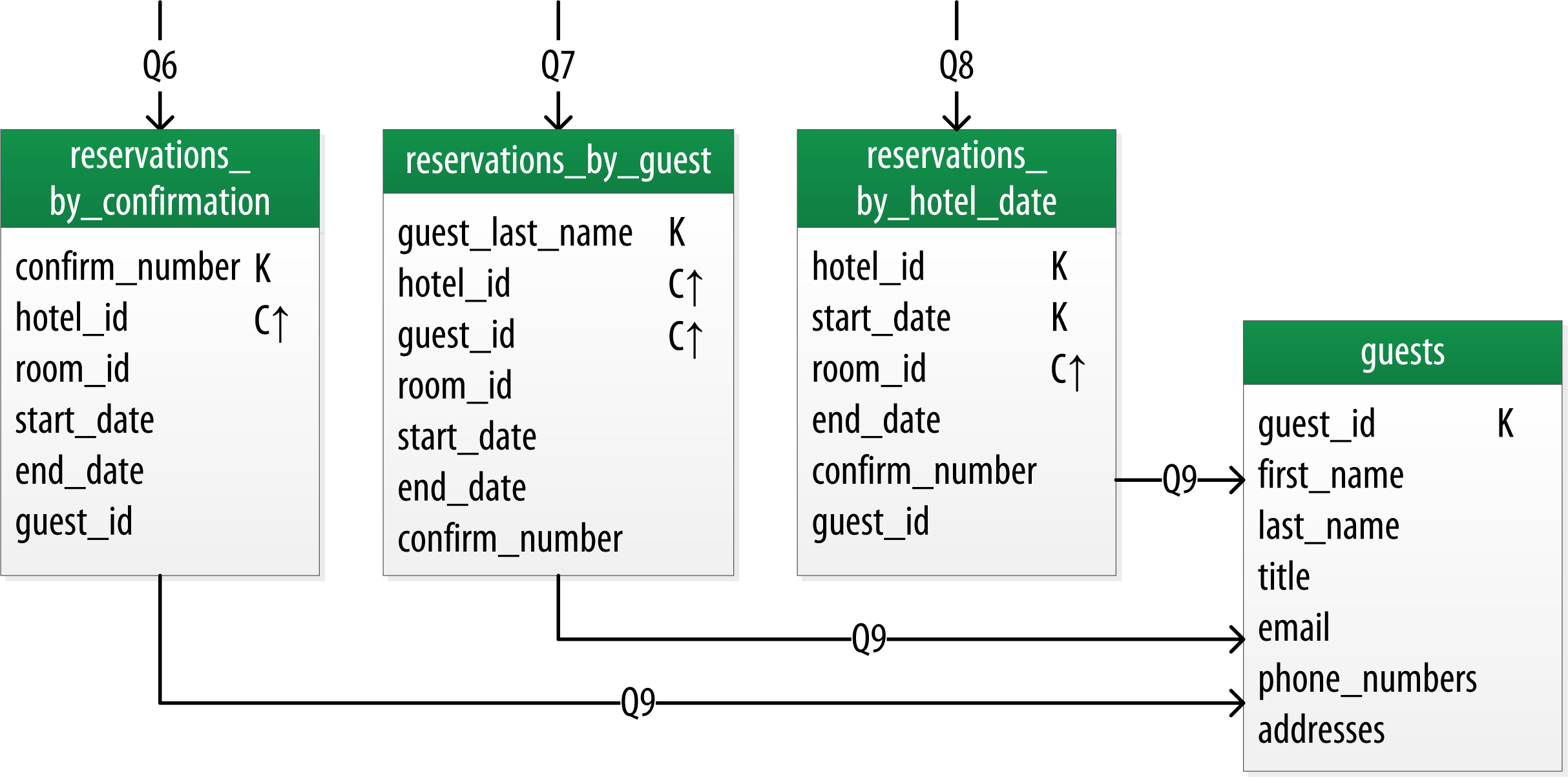
In order to satisfy Q6, the reservations_by_guest table can be used to
look up the reservation by guest name. You could envision query Q7 being
used on behalf of a guest on a self-serve website or a call center agent
trying to assist the guest. Because the guest name might not be unique,
you include the guest ID here as a clustering column as well.
Q8 and Q9 in particular help to remind you to create queries that support various stakeholders of the application, not just customers but staff as well, and perhaps even the analytics team, suppliers, and so on.
The hotel staff might wish to see a record of upcoming reservations by date in order to get insight into how the hotel is performing, such as what dates the hotel is sold out or undersold. Q8 supports the retrieval of reservations for a given hotel by date.
Finally, you create a guests table. This provides a single location
that used to store guest information. In this case, you specify a
separate unique identifier for guest records, as it is not uncommon for
guests to have the same name. In many organizations, a customer database
such as the guests table would be part of a separate customer
management application, which is why other guest access patterns were
omitted from the example.
Patterns and Anti-Patterns
As with other types of software design, there are some well-known patterns and anti-patterns for data modeling in Cassandra. You’ve already used one of the most common patterns in this hotel model—the wide partition pattern.
The time series pattern is an extension of the wide partition pattern. In this pattern, a series of measurements at specific time intervals are stored in a wide partition, where the measurement time is used as part of the partition key. This pattern is frequently used in domains including business analysis, sensor data management, and scientific experiments.
The time series pattern is also useful for data other than measurements. Consider the example of a banking application. You could store each customer’s balance in a row, but that might lead to a lot of read and write contention as various customers check their balance or make transactions. You’d probably be tempted to wrap a transaction around writes just to protect the balance from being updated in error. In contrast, a time series–style design would store each transaction as a timestamped row and leave the work of calculating the current balance to the application.
One design trap that many new users fall into is attempting to use
Cassandra as a queue. Each item in the queue is stored with a timestamp
in a wide partition. Items are appended to the end of the queue and read
from the front, being deleted after they are read. This is a design that
seems attractive, especially given its apparent similarity to the time
series pattern. The problem with this approach is that the deleted items
are now tombstones <asynch-deletes> that Cassandra must scan past in
order to read from the front of the queue. Over time, a growing number
of tombstones begins to degrade read performance.
The queue anti-pattern serves as a reminder that any design that relies on the deletion of data is potentially a poorly performing design.
Material adapted from Cassandra, The Definitive Guide. Published by O’Reilly Media, Inc. Copyright © 2020 Jeff Carpenter, Eben Hewitt. All rights reserved. Used with permission.